A categoric variable has values which can be given a label or a name (think ‘category’). Examples of categoric variables include type of car, favourite film, colours, type of material, and so on.
A continuous variable can take on any numerical value. Continuous data can be collected by counting or by measuring something. Examples of continuous variables include mass, temperature and length. A length might be measured to be 1.2 m, for example, or 1.3 m, or 1.227 m, or any value in between.
An interval is the difference between one value in a set of continuous data and the next. If we want to investigate how the temperature of a cup of hot tea changes with time, we need to measure its temperature at appropriate time intervals. An interval of one day would be unsuitable, as the tea would cool to room temperature long before we take our second measurement. At the other extreme, an interval of one second would be overkill – measuring the temperature every second would certainly tell us how the temperature of the tea decreased with time, but it would give us far more information than we need. (It would also be very tricky to do unless we had access to a data logger). A time interval of 30 seconds between readings, or one minute between readings would be more suitable in this case.
If we want to measure the value of a continuous variable, we have to select an appropriate measuring device (instrument). The resolution of a device is the smallest change that the device can detect (in the variable being measured). If the resolution of a digital watch is one second, that means one second is the smallest amount of time it can measure. The stop-clocks in your science lab might have a resolution of 0.01 seconds, which means that they can measure times of 0.01, 1.25 or 10.87 seconds (or any other time to two decimal places).
Does that mean a time that is measured using a stop-clock is always more accurate than one that’s measured using a digital watch? Well, not necessarily. Read on!
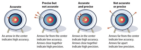
A measured value (or calculation or estimate) which is accurate is one which is close to its actual value. Let’s say you wanted to measure the temperature at which pure ice melts in your kitchen. If your first measurement of the temperature of the ice is 0.2 °C, and your second is 10.2 °C, then your first measurement is clearly the more accurate of the two, since it is much closer to the known value of 0 °C.
Two or more values which are precise are close to one another, but that doesn’t mean that accuracy and precision are the same thing. We could have measured the temperature of the melting ice three times and recorded values of 6.4, 6.2 and 6.3°C. This data is precise, because each of the values are close to one another, but they are inaccurate as they are quite far from the actual value of the temperature at which pure ice should melt in your kitchen.
Check out this graphic* which helps the difference between accuracy and precision.
In science, when we say that there’s an error in a measurement, it doesn’t necessarily mean that we’ve made a mistake. It means that the measurement which we’ve made is not exactly equal to the true value. There are a number of different types of errors which you have to know about for your GCSEs.
Random errors are unpredictable. Let’s say we measure how long it takes for a coin to drop from a height of 2 m to the ground. We might measure a time of 0.68 s on the first attempt, then values of 0.58 s and 0.64 s on the second and third attempts. Due to the limitations of our method of measurement, variations in the air flow in the room, the angle at which the coin was held and so on, the measurements which we take vary randomly.
To reduce the effect of random error on the accuracy of a measurement, we should take multiple readings and then work out the mean (average) value.
On a scatter graph, random error is what causes data points to be scattered about both sides of the best-fit line. The greater the random error in an investigation, the further the points will be scattered from the best-fit line.
When a measurement has a systematic error, it means that it is always ‘out’ (higher or lower than the true value) by the same amount. In other words, the error is consistent between readings. A systematic error is normally caused by a fault in the measuring device. For example, if 2 cm has been broken off one end of a 30 cm ruler, then it could (if you weren’t paying close attention) cause all measurements of length carried out using that ruler to be 2 cm greater than they really are. When there’s a systematic error in an investigation, the best-fit line on a graph of the data will be higher or lower than it should be.
An anomaly is a measurement which does not fit the expected trend. If an anomalous measurement was due to a mistake by the experimenter or a problem with the equipment, then the measurement should be repeated if possible (or ignored if it’s not possible to repeat it).
Finally, a zero error is a special type of systematic error which occurs when a measuring device gives a reading when the true value should be zero. For example if an electronic balance reads ‘– 29 g’ when nothing is sitting on top of it, then all mass measurements taken using the balance will be 29 g lower than their true values.
Kevin Quinn